
Python 3.15, released on 9 October 2026, ships a new built-in sampling profiler called profiling.sampling (nicknamed Tachyon). For anyone who writes data scripts, it answers the most common performance question in one command: "Which part of this notebook-turned-script is actually slow?" You do not need to change your code, install anything, or guess. You run your script under the profiler, or attach it to a job that is already running, and it tells you where the time went.
Below is how it works, the handful of commands worth remembering, and how to read the output without fooling yourself.
What a sampling profiler does differently
Python has had cProfile for years. It is a tracing profiler: it records every single function call and return. That is precise, but it slows the program down, and the slowdown is not even. Code that makes many tiny calls gets penalised far more than code that spends its time inside one big C function. In pandas work, that can make the pure-Python helper you wrote look worse than it really is next to a vectorised operation.
PEP 799, which introduced the new profiling package, puts the problem plainly: tracing "instruments every function call and return," which adds overhead, and cProfile "only observes the main thread."
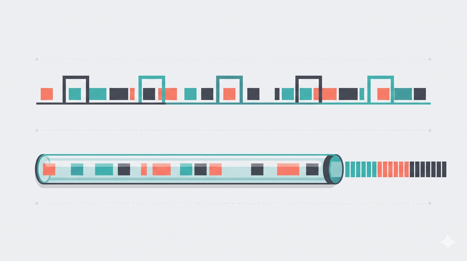
A sampling profiler works more like a photographer than a stenographer. Many times a second, it takes a snapshot of what each thread is doing and notes which function is on top of the stack. If 40% of the snapshots catch your script inside a groupby, then roughly 40% of the time is going there. The program runs at almost normal speed, because nothing is wrapped or instrumented.
In 3.15 the two approaches now sit side by side:
profiling.tracing: the deterministic profiler, relocated fromcProfile.cProfilestill works as an alias.profiling.sampling: the new statistical profiler.
The old pure-Python profile module now emits a DeprecationWarning on import and is scheduled for removal in 3.17.
Profiling a slow pandas script in one command
Say you have a script, monthly_report.py, that loads a few CSVs, cleans them and writes a summary. It takes four minutes and you want it under one. The basic run looks like this:
python -m profiling.sampling run monthly_report.pyWhen the script finishes, a table prints to the terminal. If your script takes arguments, put them after the script name and they pass straight through. A module works too:
python -m profiling.sampling run -m reports.monthly --month 2026-09For anything longer than a quick test, the flame graph is easier to read than the table:
python -m profiling.sampling run --flamegraph -o profile.html monthly_report.pyThat writes a single self-contained HTML file you can open in a browser. Width is time: the wider a block, the more samples landed in it. You can click to zoom into a function and search by file and line.
Attaching to something already running
This is the feature that will save analysts the most time. If a scheduled job has been running for 20 minutes and you want to know what it is stuck on, you do not have to kill it and start again:
python -m profiling.sampling attach --flamegraph -d 30 -o stuck.html 12345Here 12345 is the process ID, and -d 30 samples for 30 seconds and then detaches. If you just want a single snapshot of where every thread is right now, dump prints one stack trace and exits:
python -m profiling.sampling dump 12345Two catches. Attaching needs permission to read another process's memory, so on Linux you may need root or a relaxed ptrace setting, and on macOS root as well. And the profiler and the target must run the same Python minor version, so you cannot attach a 3.15 profiler to a job running on 3.12.
Wall time or CPU time: pick the right question
By default the profiler uses wall-clock mode. Every sample counts, including time spent waiting on a disk, a database or the network. Switch to CPU mode and only samples where the thread is actually computing are counted:
python -m profiling.sampling run --mode=cpu monthly_report.pyRunning both is the most useful thing you can do, because the difference tells you what kind of slow you have. The official documentation gives a neat example: a function that calls time.sleep(2) takes about 98% of samples in wall mode and vanishes entirely in CPU mode.
In a typical data script, think of it like this:
A function is big in both modes: it is genuinely computing. That is your candidate for vectorising, filtering earlier or switching to a faster engine.
A function is big in wall mode but small in CPU mode: it is waiting. Usually that means reading files, a slow SQL query or an API call. Faster pandas code will not help; caching, fewer round trips or a better query will.
There is also a --mode=gil option that only counts time while the thread holds the GIL, useful if you are experimenting with threads.
Reading the output without fooling yourself
The default table has a column called nsamples written as two numbers, such as 234/892. The first is how often the function was at the very top of the stack, doing work itself. The second is how often it was anywhere on the stack, including time spent in the functions it called.
That distinction matters. Imagine three rows from a profile of the report script, described in words:
build_report: 12 direct, 4,800 cumulative. It barely does anything itself; it just calls everything else. Ignore it.clean_addresses: 2,900 direct, 3,100 cumulative. Almost all its time is its own. This is a real hotspot, probably a row-by-rowapply.read_csv: 300 direct, 1,400 cumulative. Most time is inside pandas' parser, which is expected. Worth checking if you are reading columns you never use.
The rule from the docs: a direct-to-cumulative ratio close to 1 marks a hotspot; a big gap marks an orchestrator.
Three common mistakes to avoid:
Chasing small differences. Sample counts are estimates. The docs warn that 1 to 2% differences between runs are noise. For a precise before-and-after on one function, use
timeitor the tracing profiler.Profiling on a tiny sample. If you test on 1,000 rows, start-up and imports dominate. Profile on data that is close to the real size.
Optimising the wrong mode. If wall time is mostly I/O, a perfectly vectorised transform saves seconds out of minutes. Check CPU mode before you rewrite anything.
Should you upgrade to Python 3.15 for this?
For a personal machine or a fresh project environment, it is a reasonable reason to try 3.15, along with the UTF-8 default and the new lazy import syntax that also arrived in this release. For shared production environments, check that your key libraries publish wheels for 3.15 first; the first weeks after a release are usually when compatibility gaps show up.
A good habit to build: before you spend an afternoon rewriting a slow script, spend two minutes running it once in wall mode and once in CPU mode. More often than not, the slowest part is not the part you expected.